Occupancy Prediction and Semantic Segmentation

Introduction / Background

Humans naturally perceive the world in three dimensions, which is essential for daily activities like cooking. For robots to perform complex tasks in indoor environments, they must similarly understand the world in 3D. Traditional 3D perception requires special depth sensors that are expensive and impractical for widespread use. This necessitates the development of algorithms that can infer depth using standard cameras, despite the inherent loss of depth information in 2D images.

Recent advances in deep learning have demonstrated that this lost depth information can be recovered by leveraging geometric priors in images, large-scale datasets, and sophisticated algorithms. Beyond geometry, understanding the semantics of the environment is crucial for robots to interact effectively with their surroundings. Existing models typically predict 3D occupancy using multiview images covering a 360-degree view around a vehicle. While 3D occupancy prediction is well-researched in the context of autonomous vehicles operating outdoors, it is equally important for indoor robots [4,5,6], which face unique challenges. Building upon a recent public dataset and method for monocular occupancy prediction in indoor environments ISO [1], we aim to advance this field. This dataset comprises single-view images and voxel outputs with semantic labels for each occupied voxel. Additionally, we have decided to incorporate a smaller dataset NYUv2 which is similar to Occ-ScanNet but with less images, making it easier to train.

Description of Dataset

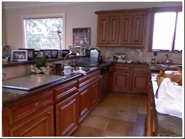
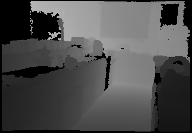
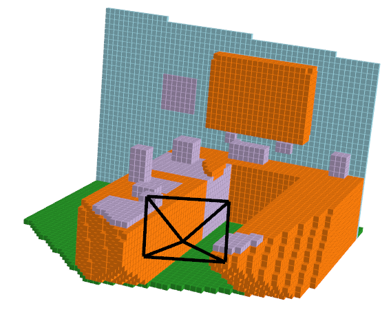
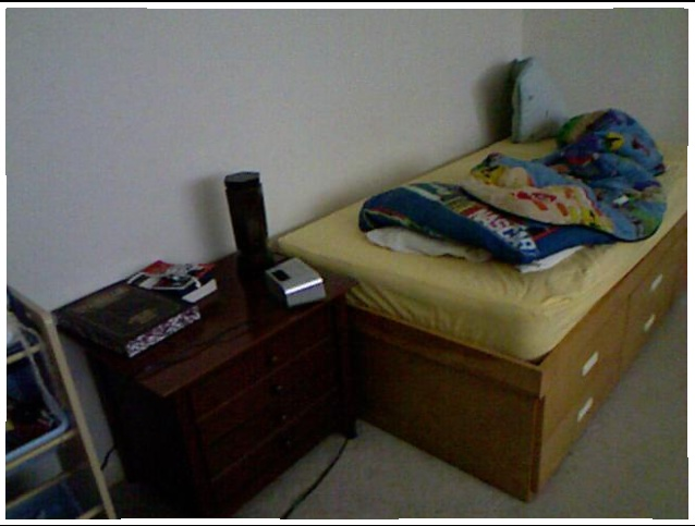
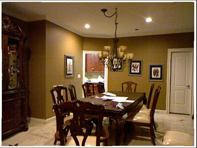
To better understand the problem, we initally did EDA to help visualize the inputs to the model and the expected outputs. Below you will see an image, a depth mask, and the expected output of the model. The depth mask is the ground truth depth mask generated from a Kinect system.

RGB Image	Depth Mask	Voxel Ground Truth

3+ References: See References

Link to Dataset: NYUv2 [8]

Problem Definition

Problem Identified: An emerging area in deep learning focuses on aligning vision and language, leading to foundational models with capabilities like open-vocabulary object segmentation. We are trying to solve three problems. Firstly, we want to generate a model that turns a 2D RGB image into a 3D voxel representation. Secondly, we want to segment the objects in the image so that we can understand the context of the scene. Thirdly, we want to label each of the segmented object in an open-vocabulary fashion.

Project Motivation: Having models that build 3D representations rich with contextual details is particularly beneficial in indoor home environments, where robots must interact with both humans and a wide variety of objects requiring fine-grained information. Since these robots ideally communicate with humans through language, employing open-vocabulary segmentation enhances their utility.

Methods

Data Preprocessing Method: PCA Compression (Unsupervised Model)

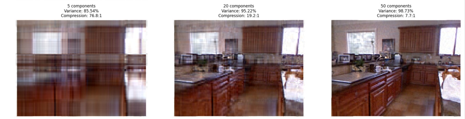
One experiment we wanted to try is seeing if PCA helps improve testing accuracy. We think PCA will help reduce the noise and highlight the most important features to input into the model. At the same time, it will hopefully have the same effect as a Gaussian blur in making the model more generalizable. Below, you can see how we used PCA to compress the NYUv2 image while selecting a good number of components to represent the structure of the image:

Model 1: MonoScene [10]

The first model we implemented was MonoScene. As of July 17, 2024, NDCSCene achieved third in performance on the NYUv2 dataset. MonoScene directly predicts 3D semantic occupancy grids from monocular images, using a voxel-based 3D representation for reconstructing dense scenes. It incorporates 3D convolutions and hierarchical refinement strategies to progressively improve spatial resolution. We set it up on the PACE cluster and trained it on a single L40S GPU for 15 epochs. The training process on the NYUv2 dataset completed within 4.2 hours. We used a learning rate of 1e-4 and applied a weight decay (regularization) of 1e-4.

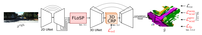
Architecture: The architecture of MonoScene starts by extracting features from a monocular input image using a 2D backbone network, typically ResNet or UNet, for visual understanding. These 2D features are lifted into 3D space via the Frustum-based Lifting module, which projects the image features into the 3D voxel space. A 3D encoder-decoder network with cascaded refinement processes these voxelized features to predict dense 3D semantic occupancy. The refinement network progressively improves the semantic accuracy and spatial detail of the reconstruction. The final output is a voxel grid, where each voxel is semantically labeled and spatially positioned, providing a full 3D representation of the input scene.

Please see Results And Discussion for how the model performed.

Model 2: NDCScene [11]

Description: The 2nd Model implemented was NDCScene [11]. As of July 17, 2024, NDCSCene achieved second in performance on the NYUv2 dataset. NDCScene transforms 2D features into NDC space instead of directly mapping to world coordinates, using deconvolution operations for progressive depth restoration. We set it up on the PACE cluster and we ran it on a single L40S GPU for 15 epochs. We were able to train it on the NYUv2 dataset within 4.6 hours. We used a learning rate of 1e-4 and a weight decay (regularization) of 1e-4.

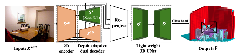
Architecture: The architecture of NDCScene processes a single image through two parallel streams: a 2D UNet that extracts visual features, and a depth branch with a pretrained depth model and DepthNet for spatial understanding. These features are merged through our specialized FLoSP (Feature Lifting and Projection) module, which helps translate 2D information into 3D space. Finally, a 3D UNet with Cascaded Refinement (CRP) transforms this combined information into a complete 3D semantic scene, where each voxel is classified and positioned correctly in the reconstructed space.

Please see Results And Discussion for how the model performed.

Model 3: ISO [1]

The third model we implemented was ISO [1]. As of July 17, 2024, ISO achieved state-of-the-art performance on the NYUv2 dataset and is the benchmark for OccScan-Net. Thus, we initially wanted to setup this model and tweak it to improve it’s performance on monocular occupancy prediction for indoor scenes. We successfully setup ISO on the PACE cluster and trained it for 15 epochs. We were able to train the model on an H100 GPU using the NYUv2 dataset within 1.5 hours. We used a learning rate of 1e-4 and a weight decay (regularization) of 1e-4.

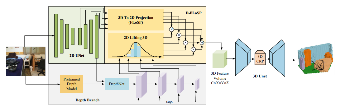
Architecture: The architecture of ISO is very similary to MonoScene. However, instead of going from a 2D UNet to a FLoSP (Feature Line of Sight Projection) segment, ISO takes the depth mask and combines it with FLoSP to create a new architecture called D-FLoSP (Dual Feature Line of Sight Projection). This enhances the 3D voxel image generated because it uses the depth to inform the model how far the voxels are from the camera. From our experiments, we can see ISO performs far better than either NDCScene or MonoScene.

Please see Results And Discussion for how the model performed.

Results and Discussion

Training / Validation model performance

The main models we were able to implement were ISO [1], NDCScene [11], and MonoScene [10]. The metrics we ended up employing were IoU, mIoU, cross entropy, precision, and recall to monitor performance.

Name	Definiton
Intersection Over Union (IoU)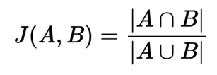
Mean Intersection Over Union (mIoU)	mIoU Definition
Cross Entropy	Cross Entropy Definition
Precision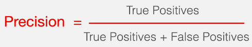
Recall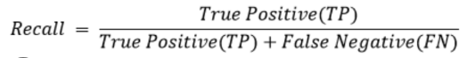

Below is the graph for IoU, mIoU, and cross entropy, precision, and recall over the training data and validation data for the 15 epoch run of MonoScene.

MonoScene Training IoU	MonoScene Validation IoU

MonoScene Training mIoU	MonoScene Validation mIoU

MonoScene Training Cross Entropy	MonoScene Validation Cross Entropy

MonoScene Training Precision	MonoScene Validation Precision

MonoScene Training Recall	MonoScene Validation Recall

Please see the following public WandB project for further metrics.

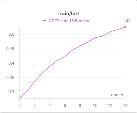
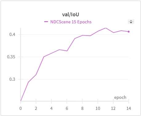
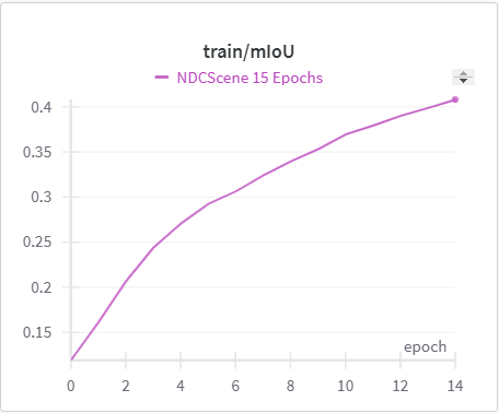
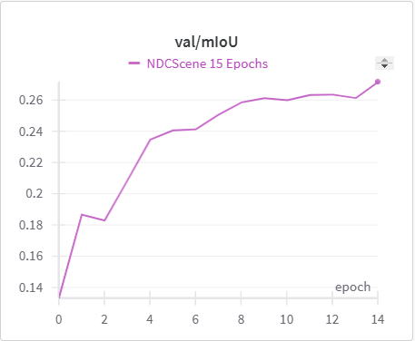
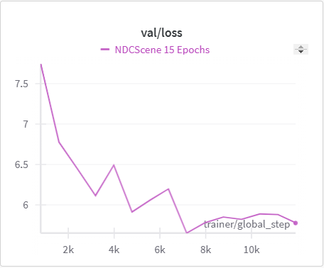
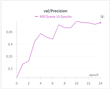
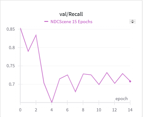
Below is the graph for IoU, mIoU, and cross entropy, precision, and recall over the training data and validation data for the 15 epoch run of NDCScene.

NDCScene Training IoU	NDCScene Validation IoU

NDCScene Training mIoU	NDCScene Validation mIoU

NDCScene Training Cross Entropy	NDCScene Validation Cross Entropy

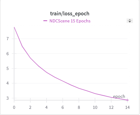NDCScene Training Precision	NDCScene Validation Precision

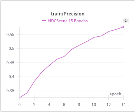NDCScene Training Recall	NDCScene Validation Recall

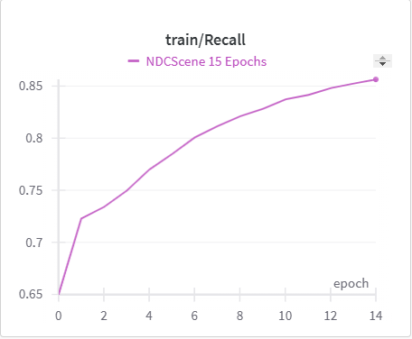Please see the following public WandB project for further metrics.

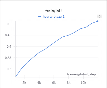
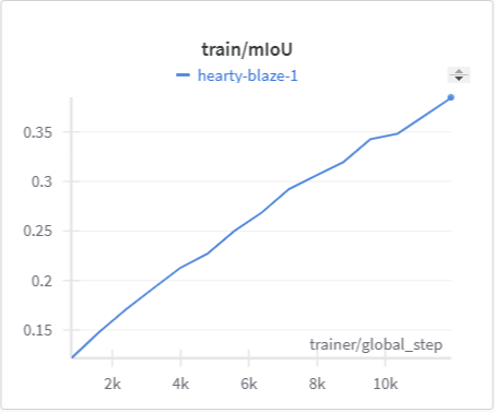
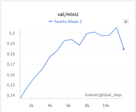
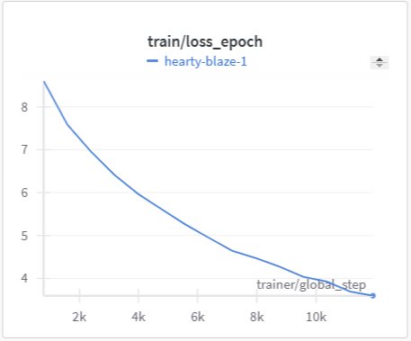
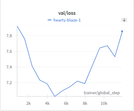
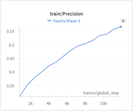
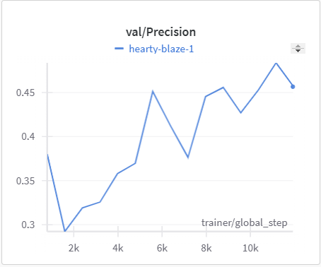
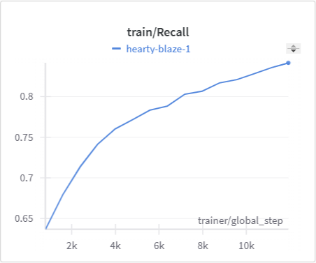
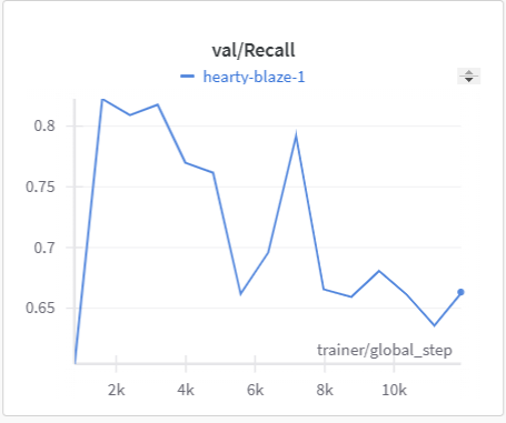
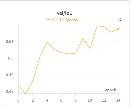
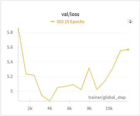
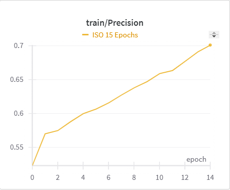
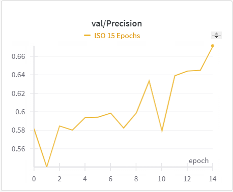
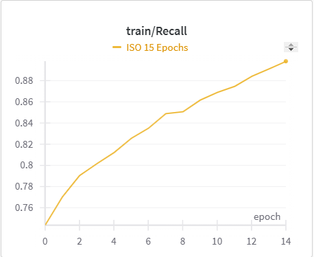
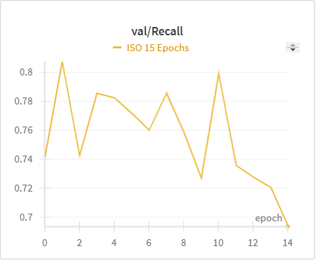
Below is the graph for IoU, mIoU, and cross entropy, precision, and recall over the training data and validation data for the 15 epoch run of ISO.

ISO Training IoU	ISO Validation IoU

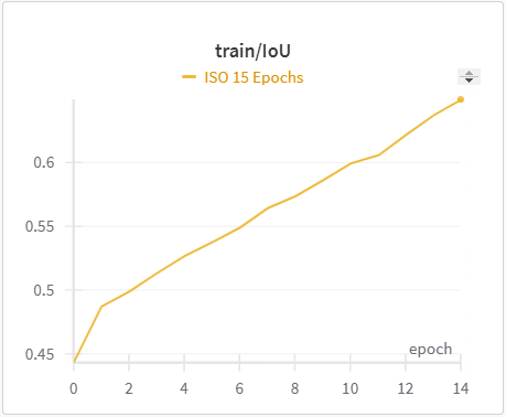ISO Training mIoU	ISO Validation mIoU

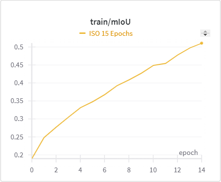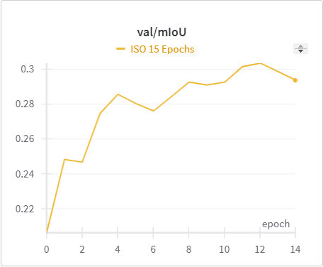ISO Training Cross Entropy	ISO Validation Cross Entropy

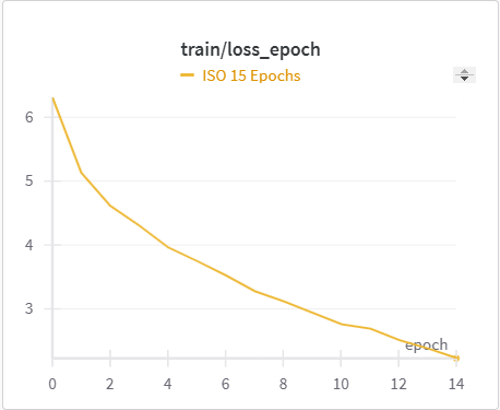ISO Training Precision	ISO Validation Precision

ISO Training Recall	ISO Validation Recall

Please see the following public WandB project for further metrics.

The IoU, mIoU, and precision improved nicely through our training run. However, the cross entropy increased and the recall decreased during some of our training runs. There are a few things that we think contributed to this issue:

1. Class imbalances, as smaller items are easier to miss (tvs and objects vs. floor and beds )
2. Need more regularization to reduce the possibility of overfitting the model to the training data (possibly earlier stopping)
3. Change thresholds when it comes to class predictions dynamically for each class

Performance Comparison (with and without PCA)

In regards to performance, we will start with the results from the original papers [1,10,11].

Original Papers Performance

Method	IoU	ceiling	floor	wall	window	chair	bed	sofa	table	tvs	furniture	object	mIoU
MonoScene	42.51	8.89	93.50	12.06	12.57	13.72	48.19	36.11	15.13	15.22	27.96	12.94	26.94
NDC-Scene	44.17	12.02	93.51	13.11	13.77	15.83	49.57	39.87	17.17	24.57	31.00	14.96	29.03
ISO	47.11	14.21	93.47	15.89	15.14	18.35	50.01	40.82	18.25	25.90	34.08	17.67	31.25

Next, we will compare it to our performance we received when running the models on the NYU dataset.

Our Performance on NYU Dataset without PCA

Method	IoU	ceiling	floor	wall	window	chair	bed	sofa	table	tvs	furniture	object	mIoU
MonoScene	37.07	5.12	93.32	9.61	6.27	9.96	16.49	19.76	10.43	3.34	20.87	7.84	18.46
NDC-Scene	39.99	7.93	93.41	10.55	8.80	12.52	43.72	34.56	15.42	16.63	26.89	11.89	25.67
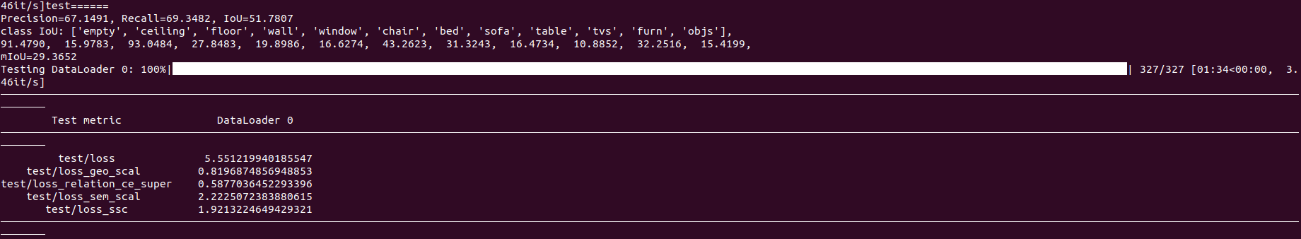
ISO	51.78	15.98	93.05	27.85	19.90	16.63	43.26	31.32	16.47	10.88	32.25	15.42	29.37

As you can see, our own runs for MonoScene and NDC-Scene underperformed from what the original paper’s values were. We think this is three fold:

1. Random initialization was different from what the original papers used
2. We did not tune the hyperperameters of the model (due to time constraints)
3. Stopping early at 15 epochs (from early experiments, we thought it would help with regularization)

However, we did improve upon the score in the ISO paper when it comes to IoU and a few of the categories. This was mainly due to the following:

1. Changing the backbone from ConvNext to EfficientNet (a better, more efficient model)
2. Using the ground truth labels for depth, as given by the Kinect system

Our Performance on NYU Dataset with PCA

Method	IoU	ceiling	floor	wall	window	chair	bed	sofa	table	tvs	furniture	object	mIoU
MonoScene	34.09	6.76	93.50	8.53	6.19	7.54	20.27	15.72	6.56	3.11	13.79	7.86	17.26
NDC-Scene	40.14	6.13	93.45	11.10	12.34	14.22	45.34	35.81	16.00	15.44	28.11	12.12	26.37
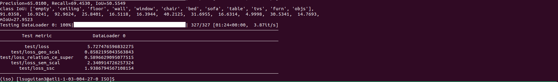
ISO	50.55	16.92	92.96	25.84	16.51	16.39	40.21	31.70	16.63	5.00	30.53	14.77	27.95

Experiment 1 Results: Unfortunately, adding PCA did not help with model validation accuracy for ISO and MonoScene. It did slightly improve results for NDCScene. This is likely because NDC Scene relies on projecting to the normalized device coordinate (NDC) space instead of directly to world space coordinates, allowing it to gather more rich information from the PCA images.

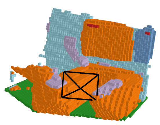
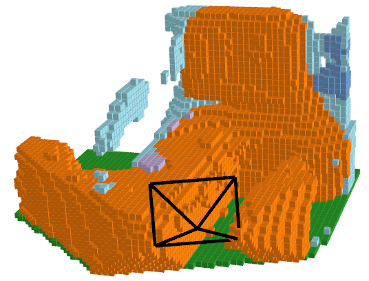
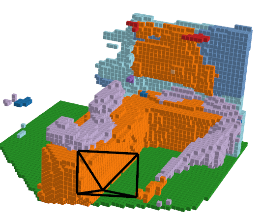
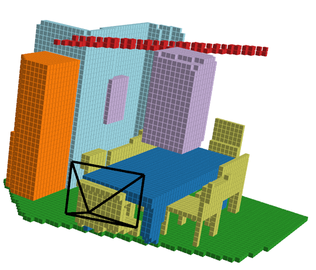
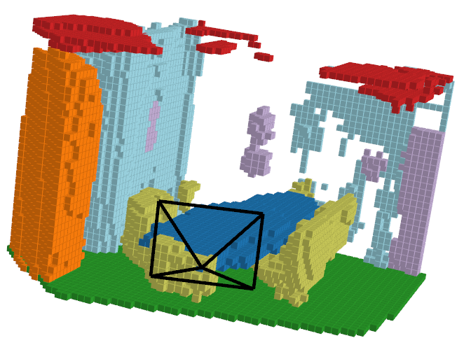
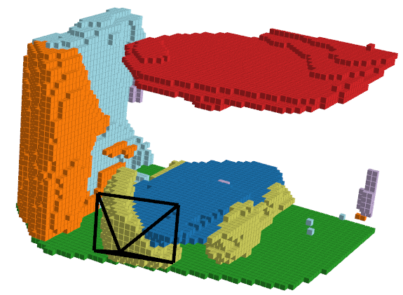
Let’s take a look at an example of what the predicted outputs look like:

RGB Image	Ground Truth	ISO Prediction	NDCScene Prediction	MonoScene Prediction

RGB Image	Ground Truth	ISO Prediction	NDCScene Prediction	MonoScene Prediction

RGB Image	Ground Truth	ISO Prediction	NDCScene Prediction	MonoScene Prediction

AutoEncoder and Open Vocabulary experiments

Semantic Sam

Our ultimate goal is to build a model that operates on semantic categories rather than individual instances. Therefore, after the midterm phase of this project, we transitioned from using the original Segment Anything Model (SAM) [2] to Semantic SAM for image segmentation. While SAM excels at part-level segmentation, it often leads to over-segmentation, producing fragmented results that are not ideal for learning object-level features. Semantic SAM [12], built upon the foundation of SAM, addresses this limitation by providing segmentation at multiple granularities, yielding more coherent and semantically meaningful masks. This coherence is crucial for ensuring that our final voxel-based model can effectively learn features corresponding to actual objects.

Consequently, we adopted Semantic SAM [12] and preprocessed our entire dataset to obtain high-quality segmentation masks for all images. It is important to note that, similar to SAM, Semantic SAM primarily focuses on mask prediction and does not inherently classify the semantic category of the objects within those masks. To address this, we employ open vocabulary classification models, as detailed in the following section, to predict the semantic category associated with each segmented mask.

Open Vocabulary Classification

1. Introduction to Open Vocabulary Classification

Traditional approaches to object classification and recognition rely on closed-vocabulary models. These models are trained on predefined sets of labeled data, typically encompassing a limited range of categories (e.g., 10-100 classes). For instance, the OccScanNet dataset, which we utilize in this work, contains only 12 generic classes such as “floor,” “ceiling,” and “furniture.” However, for robots to effectively operate and collaborate with humans in real-world environments, the ability to understand and respond to natural language instructions is crucial. This necessitates the capacity to perceive and identify objects using arbitrary language specified by the user.

Recent advancements in large-scale vision-language models, such as CLIP and SigLIP [13], have paved the way for open-vocabulary classification. These models are trained on massive datasets of image-text pairs (around 500 million pairs), exhibiting emergent capabilities to classify objects based on textual descriptions. This allows for queries like “sofa,” “MacBook,” or even more descriptive phrases like “cup with a blue handle.” In essence, open vocabulary classification empowers models to recognize objects based on user-defined, free-form language queries.

2. Methodology

2.1. Open Vocabulary Model

To achieve open-vocabulary capabilities in our system, we leverage the Semantic SAM model [12] for mask prediction, followed by SigLIP for category classification. SigLIP [13] was chosen over CLIP due to its superior performance in our preliminary experiments and was adopted as our primary model after the midterm phase of this project.

2.2. Vocabulary Selection for Indoor Environments

While our model is designed for open vocabulary classification, practical constraints on computational resources necessitate a finite vocabulary. Therefore, we curated a vocabulary of 250 object categories relevant to indoor scenes. This vocabulary was derived from the LVIS dataset, and we utilized ChatGPT to filter and select categories most likely to occur in indoor environments. We acknowledge that this is not a truly “open” vocabulary encompassing all possible nouns in the English language. However, the methodology we present is readily extensible to incorporate a larger vocabulary, enabling a truly open-vocabulary system in the future.

2.3. Object Classification and Embedding Generation

The masks predicted by Semantic SAM are sequentially processed by SigLIP. SigLIP predicts a category label from our predefined 250-class vocabulary and generates a 1152-dimensional embedding vector for each masked image. These embeddings serve as input features for our ISO model, which is further discussed in the following sections. The ISO model leverages these embeddings to enhance category prediction and scene understanding.

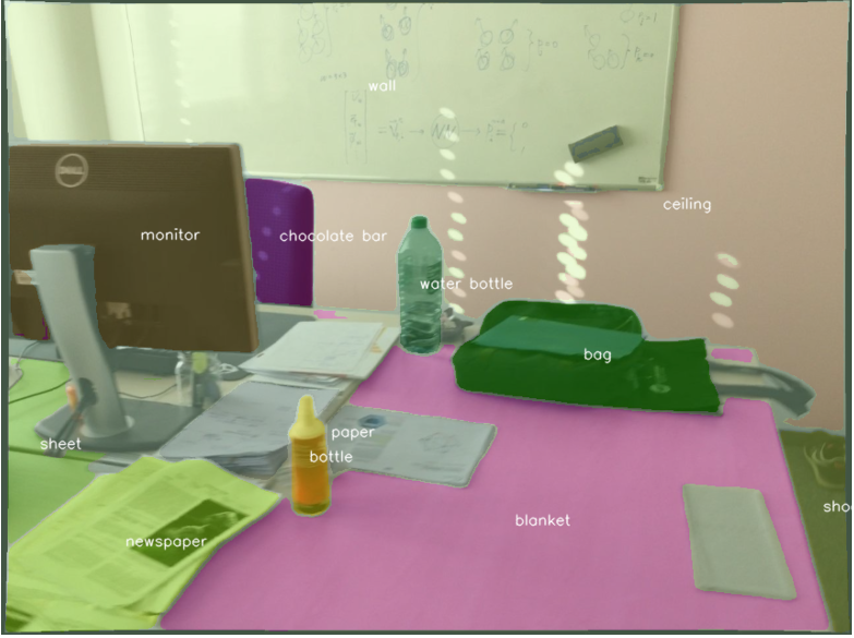
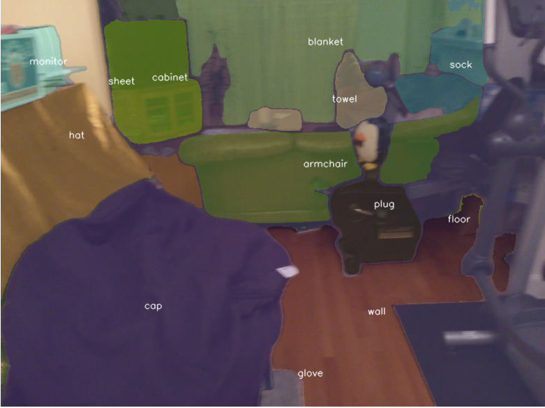
This image shows the openvocab nature, although inaccurate, we are still able to capture very specific details like “newspaper”, shoes which can be very useful in domestic robots.

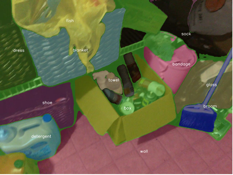
In this image also objects like detergent and broom are detected separately, which is not trivial to solve in closed vocabulary setting.

AutoEncoder

As previously established, SigLIP generates 1152-dimensional embedding vectors. To integrate these embeddings with our Implicit Scene Occupancy (ISO) model, we initially considered concatenating SigLIP’s output directly with the feature maps extracted by the ISO encoder. However, this approach results in a dense tensor of size h x w x 1152 (height x width x 1152), significantly increasing computational cost and memory requirements. To mitigate this issue, we employ an autoencoder to reduce the dimensionality of the SigLIP embeddings from 1152 to a lower-dimensional space |d|, where |d| « 1152. Through experimentation with various embedding dimensions, we found that |d| = 64 provides an optimal balance between dimensionality reduction and classification accuracy. The table below presents the classification performance achieved with different embedding sizes, compared against the upper bound performance obtained using the full 1152-dimensional embeddings. This demonstrates the effectiveness of our autoencoder-based dimensionality reduction approach.

Hidden Dimension Size	Classification Accuracy (Higher is better)
1152 (Upper bound)	67.8 %
32	60.7 %
64	63.6 %
128	64.4 %
512	65.8 %

67% accuracy is reasonable zero shot accuracy especially considering the number of classes is 253.

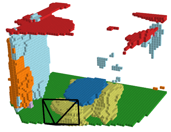
Open Vocabulary Voxel Creation

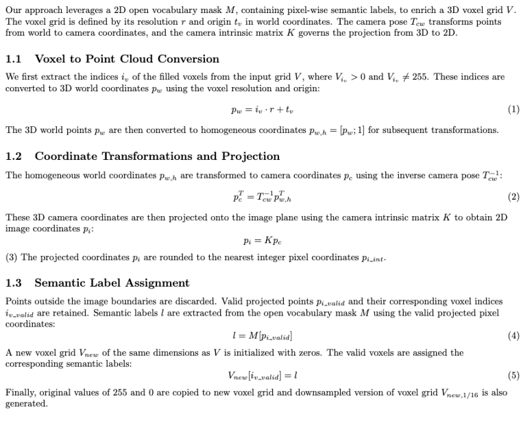
Once we obtain open vocabulary mask, we also need steps to convert it to voxels. This algorithm is described in detail here, we also show the results of open vocabulary vs original voxels here. The algorithm takes a 3D voxel representation of a scene and enhances it with semantic information from a corresponding 2D image that has been pre-labeled with object categories (an “open vocabulary mask”). First, each filled voxel in the 3D model is converted into a 3D point in world coordinates. Then, using camera intrinsics, these 3D points are projected onto the 2D image plane, effectively simulating how the scene would appear from the camera’s viewpoint. For each projected point, the algorithm checks the corresponding pixel label in the 2D mask. This label, indicating the object category at that pixel (e.g., “chair,” “table”), is then assigned to the original voxel. Finally, a new 3D voxel grid is created where each voxel retains its original spatial location but now possesses the semantic label derived from the 2D image. This process effectively colors the 3D model with semantic information, creating a more informative and contextually rich scene representation.

Open Vocabulary Classification - Results

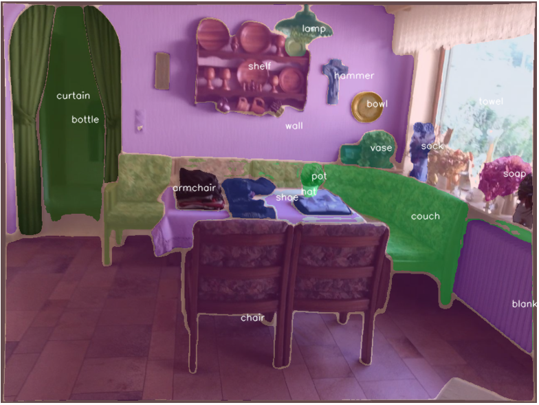
Images with open vocabulary mask

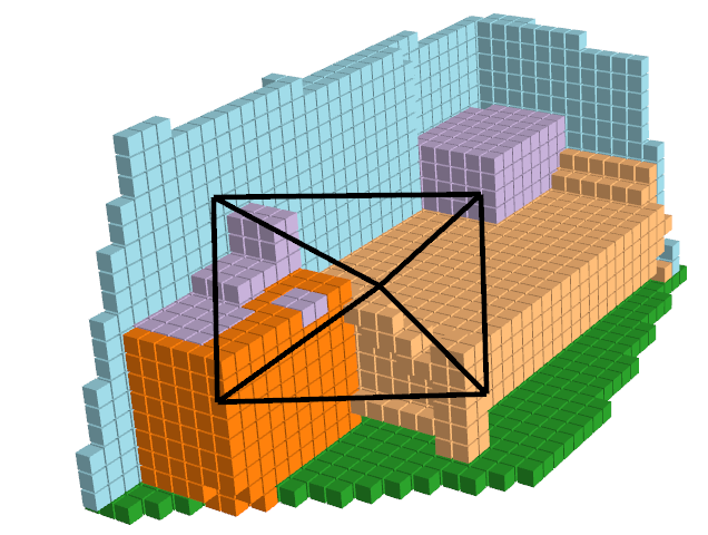
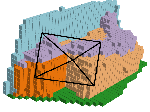
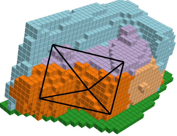
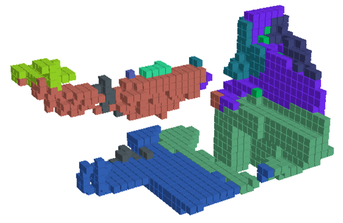
Open Vocabulary Voxels

Original Voxel Predictions

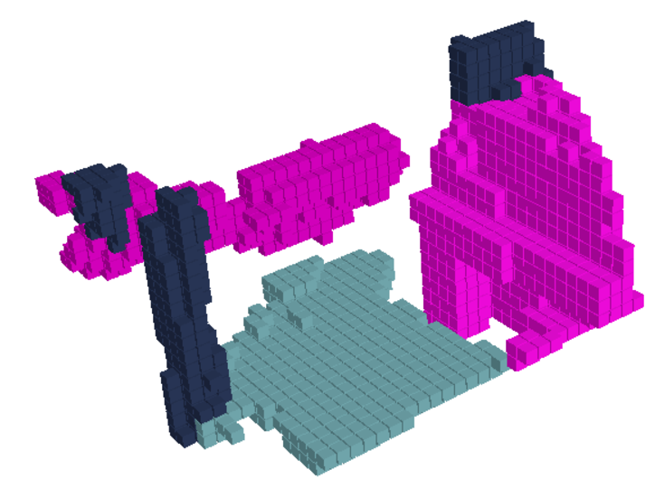
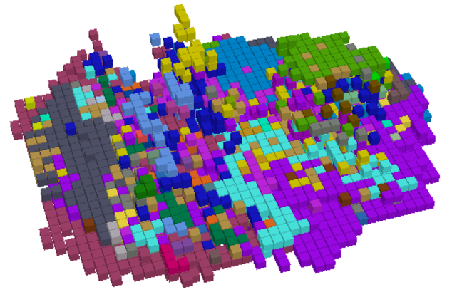
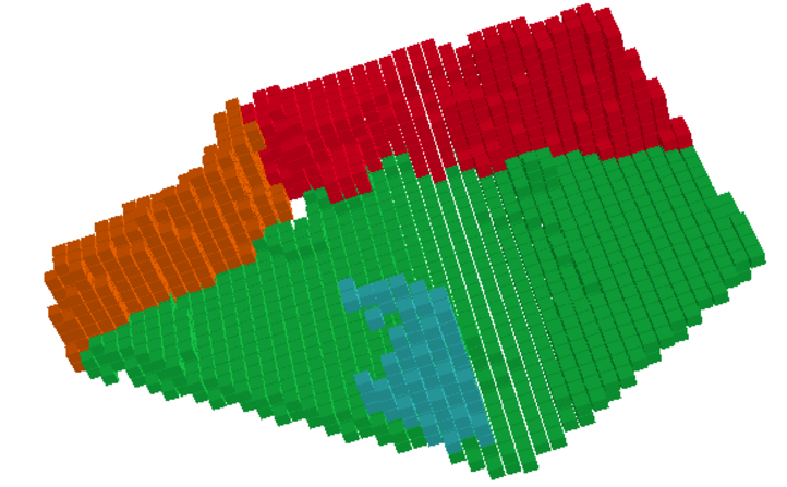
Understanding these figures are little challenging, lets discern it, the pink voxels in second figure belong to furniture class, all the objects are labeled sofa in original, on the other hand in open vocabulary voxel, we see that the voxels are subdivided, brown colored voxels belong to armchair. The cabinet in the back is labeled as “object” in original voxel, which can be seen in light green color in the open vocab voxel.

Integrating with ISO

Directly training a model to predict 256 semantic classes from scratch is a challenging task, particularly with limited data. This difficulty is well-documented in the literature, where zero-shot performance of models pre-trained on large datasets often surpasses that of models trained exclusively on datasets like LVIS, which suffer from class imbalance (some classes having as few as 5 samples). To address this challenge and leverage the knowledge encoded in large-scale vision-language models, we integrate the embeddings extracted by SigLIP into our ISO model as supplementary feature maps. This integration can be conceptualized as incorporating an “external expert” that provides 2D semantic predictions, which the ISO model then lifts to 3D voxel space. Essentially, the SigLIP embeddings provide valuable semantic cues to guide the ISO model’s predictions.

While our experiments yielded promising Intersection over Union (IoU) scores of approximately 0.2, we observed instances of the model predicting spurious classes in some voxels. We hypothesize that this behavior stems from the relatively small size of our training dataset (1000 images) and that effectively leveraging these rich feature maps requires a substantially larger dataset. Although a dataset of 45,000 images is available, training on such a scale demands significant computational resources and time. Therefore, we leave the exploration of larger datasets and the extension of this work to a truly open vocabulary as future research directions.

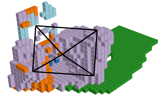
Our Autoencoder with ISO - Open Vocabulary

Original ISO Prediction - Limited Vocabulary

As seen in first image, model is almost able to pick up the geometry of the scene, but learning semantics from 64 dimensional feature map needs more training. We suspect training on larger dataset for more iterations should solve the issue.

Next Steps:

1. Change PCA hyperparameters to see if more / less compression helps improve testing results
2. Expand open-vocabulary beyond our 255 nouns
3. See if hyperparameter tuning can improve the models
4. Train ISO on the full Occ-ScanNet dataset and use transfer learning on NYUv2 to improve performance

References

[1] H. Yu, Y. Wang, Y. Chen, and Z. Zhang, “Monocular Occupancy Prediction for Scalable Indoor Scenes”. 2024. [Online]. Available: https://arxiv.org/abs/2407.11730

[2] A. Kirillov, E. Mintun, N. Ravi, H. Mao, C. Rolland, L. Gustafson, T. Xiao, S. Whitehead, A. Berg, W. Lo, P. Dollár, and R. Girshick. “Segment Anything”. 2023. [Online]. Available: https://arxiv.org/pdf/2304.02643

[3] A. Radford, J. Kim, C. Hallacy, A. Ramesh, G. Goh, S. Agarwal, G. Sastry, A. Askell, P. Mishkin, J. Clark, G. Krueger, and I. Sutskever. “Learning Transferable Visual Models From Natural Language Supervision”. 2021. [Online]. Available: https://arxiv.org/abs/2103.00020

[4] A. Vobecky, O. Siméoni, D. Hurych, S. Gidaris, A. Bursuc, P. Pérez, and J. Sivic. “POP-3D: Open-Vocabulary 3D Occupancy Prediction from Images”. 2024. [Online]. Available: https://arxiv.org/abs/2407.11730

[5] M. Qin, W. Li, J. Zhou, H. Wang, and H. Pfister. “LangSplat: 3D Language Gaussian Splatting”. 2024. [Online]. Available: https://arxiv.org/abs/2312.16084

[6] C. Chen, R. Wang, Y. Guo, C. Zhao, X. Huang, C. Feng, and L. Ren. “AdaOcc: Adaptive-Resolution Occupancy Prediction”. 2024. [Online]. Available: https://arxiv.org/abs/2408.13454

[7] Y. Li, Z. Yu, C. Choy, C. Xiao, J. Alvarez, S. Fidler, C. Feng, and A. Anandkumar. “VoxFormer: Sparse Voxel Transformer for Camera-based 3D Semantic Scene Completion”. 2024. [Online]. Available: https://arxiv.org/abs/2302.12251

[8] N. Silberman, D. Hoiem, P. Kohli, and R. Fergus. “Indoor Segmentation and Support Inference from RGBD Images” in ECCV, 2012. [Online]. Available: https://cs.nyu.edu/~fergus/datasets/indoor_seg_support.pdf

[9] A. Ganj, H. Su, and T. Guo. “HybridDepth: Robust Metric Depth Fusion by Leveraging Depth from Focus and Single-Image Priors”. 2024. [Online]. Available: https://arxiv.org/abs/2407.18443

[10] A. Cao and R. de Charette. “MonoScene: Monocular 3D Semantic Scene Completion”, 2022. [Online]. Available: https://arxiv.org/abs/2112.00726

[11] J. Yao, C. Li, K. Sun, Y. Cai, H, Li, W. Ouyang and H. Li. “NDC-Scene: Boost Monocular 3D Semantic Scene Completion in Normalized Device Coordinates Space”. 2023. [Online]. Available: https://arxiv.org/abs/2309.14616

[12] F. Li, H. Zhang, P. Sun, X. Zou, S. Liu, J. Yang, C. Li, L. Zhang and Jianfeng Gao. “Semantic-SAM: Segment and Recognize Anything at Any Granularity”. 2023. [Online]. Available: https://arxiv.org/abs/2307.04767

[13] X. Zhai, B. Mustafa, A. Kolesnikov and L. Beyer. “Sigmoid Loss for Language Image Pre-Training”. 2023. [Online]. Available: https://arxiv.org/abs/2303.15343

Gantt Chart

Gantt Chart: Click here to download

Contribution Table

Name	Proposal Contributions
Yash Bhalchandra	SAM/CLIP setup and pipeline implementation. Autoencoder build out.
Vishrut Goel	PCA setup and implementation. NDCScene setup.
Mainak Mallick	MonoScene setup and implementation.
Logan Suguitan	GitHub pages and Gantt chart setup. ISO model setup and implementation. NDCScene setup and implementation.
Sanchit Tanwar	Selected model strategy and design. Adding ISO enhancements. Open-vocab implementation.

GitHub Repo

GitHub Repo

Appendix

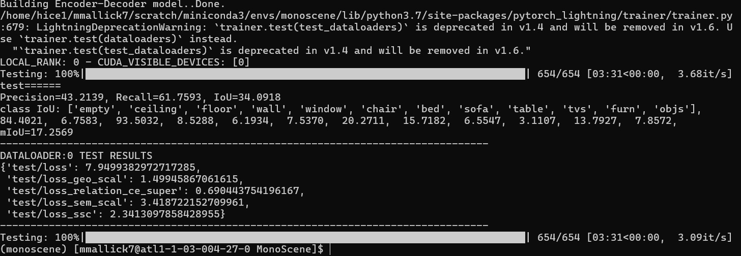
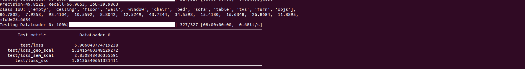
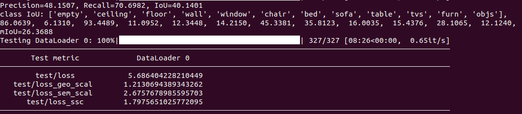
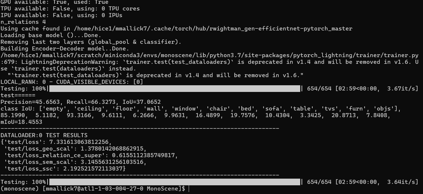
Here is a print out of the results we received as confirmation of our own runs:

ISO no PCA

ISO with PCA

NDCScene no PCA

NDCScene with PCA

MonoScene no PCA

MonoScene with PCA